Velocity

How Does Radar Measure Velocity?

The mmWave Core does not normally measure velocity by calculating how much an object’s displayed distance changes between frames. Instead, it detects extremely small changes in the phase of the reflected radar signal.

How does this work?

A useful way to think about phase is as the position within one cycle of a wave. If an object moves slightly between two chirps, the radar wave must travel a slightly different round-trip distance. This causes the returned wave to arrive at a different point in its cycle.

The radar wave travels:

1. From the radar to the target
2. From the target back to the radar

Suppose the target moves slightly closer between two chirps.

The second reflected signal travels a slightly shorter distance. Because it travels a shorter distance, it completes a slightly different number of wave cycles before arriving back at the radar.

That causes the second return to arrive at a different point in its cycle.

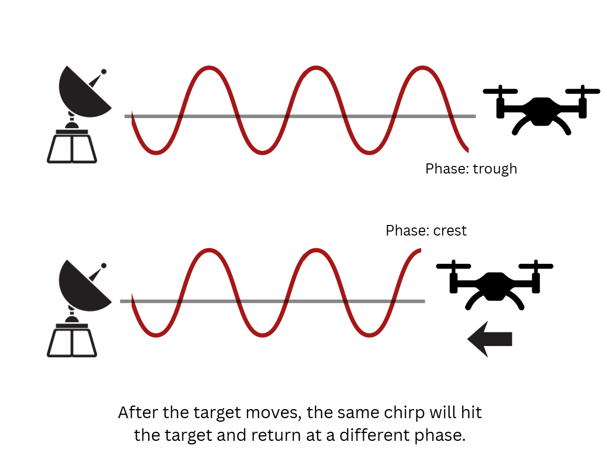
The measurement process can be summarized as follows:

1. The radar transmits one chirp.
2. The chirp reflects from an object and returns to the radar.
3. The radar processes the return to determine the object’s range and the phase of its signal.
4. The radar transmits another (identical) chirp a short time later.
5. If the object has moved toward or away from the radar, the phase of its return changes.
6. The radar measures the rate of phase change across many chirps and converts it into radial velocity.

For two measurements separated by a time $T_r$, the phase change is

$$\Delta \phi = \frac{4\pi v_r T_r}{\lambda}$$

and the radial velocity can be calculated as

$$v_r = \frac{\lambda \Delta \phi}{4\pi T_r}$$

where:

• ($v_r$) is radial velocity,
• ($\lambda$) is the radar wavelength,
• ( $T_r$) is the time between observations made by the same transmitter,
• ($\Delta\phi$) is the measured phase change.

Because the AWR2944 operates around 76–81 GHz, its wavelength is only a few millimeters. Even a very small change in target position can therefore create a measurable phase change.

Radial Velocity

The velocity reported by the radar is radial velocity: the part of an object’s motion that is directly toward or away from the radar.

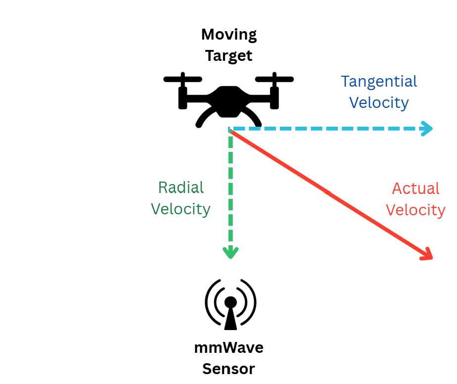
If an object is moving at speed ($v$) at an angle ($\theta$) relative to the radar’s line of sight, the measured velocity is approximately

$$v_r = v\cos(\theta)$$

An object flying directly toward the radar produces a large radial velocity. The same object flying directly sideways across the radar’s field of view may have a radial velocity close to zero, even though its actual speed is high.

Tracking software can estimate two-dimensional motion by combining radial velocity with changes in position over multiple frames, but the instantaneous Doppler measurement itself is radial.

What Is Doppler?

The Doppler effect is the change observed in a wave when the distance between the source and the observer is changing.

A familiar example is the sound of a vehicle siren:

• As the vehicle approaches, the sound waves arrive more quickly and the pitch appears higher.
• As the vehicle moves away, the waves arrive less quickly and the pitch appears lower.

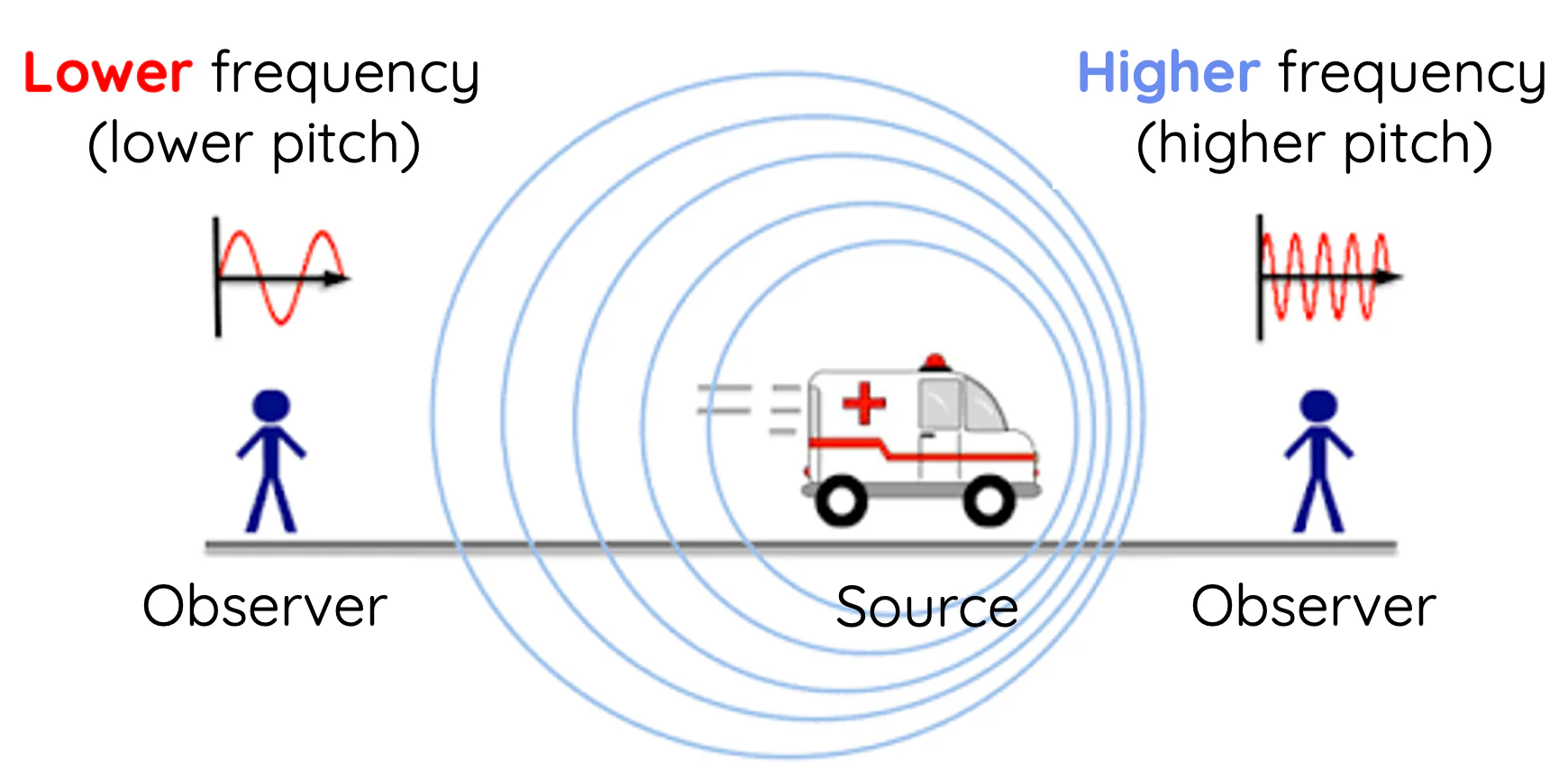
Radar experiences the same general effect with electromagnetic waves. A target moving toward the radar shifts the returned signal in one direction, while a target moving away shifts it in the opposite direction.

The Doppler frequency produced by a target is

$$f_D = \frac{2v_r}{\lambda}$$

or, rearranged,

$$v_r = \frac{\lambda f_D}{2}$$

The factor of two appears because the radar wave travels from the radar to the target and then back again.

In an FMCW radar such as the mmWave Core, Doppler is commonly measured by observing phase progression across repeated chirps. The radar first performs a range FFT to separate reflections by distance. It then performs a Doppler FFT across the chirps for each range location. The result is an array that can be represented as a range-Doppler heatmap, in which one axis represents distance and the other represents radial velocity.

What is FFT?

An FFT, or Fast Fourier Transform, is a mathematical tool that separates a mixed signal into its individual frequency components. In radar processing, the range FFT analyzes the samples collected during each chirp and converts them into range bins, where each bin represents a different distance from the radar. The Doppler FFT then compares the signal across multiple chirps and separates targets into velocity bins based on how their signal phase changes over time. Together, these two steps allow the radar to determine both where a target is and how quickly it is moving toward or away from the radar.

A target with no radial motion appears near the zero-Doppler bin. A moving object appears in a positive or negative Doppler bin, depending on the sign convention used by the software.

Objects with rotating or vibrating components can produce several Doppler components at once. For example, a drone body may produce a velocity close to the aircraft’s overall radial velocity, while its rotating propellers produce additional micro-Doppler signatures around that velocity.

Maximum Velocity vs. Velocity Resolution

You may have heard of two ways to characterize a mmWave Radar’s velocity measurement capabilities: maximum velocity and velocity resolution. These are two different measurements, just like range and range resolution.

Maximum Unambiguous Velocity

The maximum unambiguous velocity is the highest radial speed that can be uniquely determined from the chirp-to-chirp phase change.

Why?

If a target exceeds this limit, the target does not necessarily disappear. Instead, its measured velocity may wrap, or alias, into the supported velocity interval. This is very similar to when a camera doesn’t capture frames fast enough: A fast target may therefore appear to be moving at a slower speed or even in the wrong direction.

Higher-level velocity-disambiguation and tracking algorithms can sometimes recover speeds beyond the native unambiguous limit, but this depends on the waveform and processing implementation.

For a conventional evenly spaced chirp sequence,

$$v_{\max} = \frac{\lambda}{4T_r}$$

A shorter time between measurements allows the radar to measure a larger unambiguous velocity.

Velocity Resolution

Velocity resolution is the minimum radial-velocity separation needed for two targets at approximately the same range to appear in separate Doppler bins.

For a conventional chirp sequence,

$$\Delta v = \frac{\lambda}{2N_D T_r}$$

where $N_D$ is the number of chirp observations from the same transmitter used in the Doppler FFT.

The equation may also be written as

$$\Delta v = \frac{2v_{\max}}{N_D}$$

A smaller value of $\Delta v$ represents better velocity resolution.

Increasing the number of chirps increases the total observation time and produces more closely spaced Doppler bins. TI therefore describes velocity resolution as primarily dependent on the active transmit or observation time of the frame.

Resolution Is Not the Same as Accuracy

Velocity resolution describes the spacing between Doppler bins. It does not guarantee that every velocity measurement will have exactly that error.

Actual velocity accuracy also depends on factors such as:

• Signal-to-noise ratio
• Target strength and orientation
• Interference and multipath reflections
• Phase noise
• Target acceleration during the measurement
• FFT windowing and peak interpolation
• Detection and tracking algorithms

A tracker may report values between the raw Doppler-bin centers, but that does not mean the radar has gained the ability to resolve two targets separated by less than the underlying Doppler resolution.

What Affects Velocity Measurements?

Chirp Cycle Time

For one chirp, the cycle time is approximately

$$T_{\text{chirp}} = \text{idleTime}+\text{rampEndTime}$$

These values are configurable through the mmWave Core API.

Reducing either parameter can shorten the chirp cycle and increase maximum unambiguous velocity. However, the values cannot be reduced without considering RF settling time, ADC collection time and the required frequency sweep.

Why?

A chirp can be viewed as the following sequence:

1. The previous frequency sweep ends.
2. The radar returns to the starting frequency during a set idle time.
3. A new frequency sweep begins.
4. The radar waits for the transmitted and received signals to stabilize.
5. The ADC records the reflected signal.
6. The sweep ends and the process repeats.

RF Settling Time

The radar does not change frequency instantaneously. At the end of a chirp, its frequency synthesizer must return from the final chirp frequency to the starting frequency of the next chirp. It then needs enough time to settle at that frequency.

This reset and settling process occurs primarily during idleTime. If idleTime is too short, the next chirp may begin before the synthesizer has fully returned to the correct starting frequency. The resulting chirp may have an incorrect starting frequency or a nonlinear frequency sweep. The required settling time generally increases when the chirp covers a larger frequency bandwidth.

There is also a second settling period at the beginning of the ramp. When the new sweep begins, the phase-locked loop, transmitter, receiver and analog filters need a short amount of time to reach stable operation. The ADC therefore does not normally begin recording immediately when the ramp starts. Instead, it waits for the configured adcStartTime.

Starting the ADC too early may capture the unstable beginning of the chirp. This can distort the recorded signal and degrade range and Doppler processing. The required adcStartTime depends on factors such as frequency slope, filter configuration and ADC sampling mode. TI specifically notes that the time required for the AWR2944 chirp to become linear depends on its frequency slope.

ADC Collection Time

Once the signal has settled, the ADC must have enough time to collect every configured sample.

The ADC collection time is

$$T_{\text{ADC}} = \frac{N_{\text{ADC}}}{f_s}$$

where:

• $N_{\text{ADC}}$ is the number of ADC samples per chirp.
• $f_s$ is the ADC sampling rate.

For example, collecting 256 samples at 10 million samples per second requires $25.6\ \mu\text{s}$

Because rampEndTime is measured from the beginning of the frequency ramp, it must be long enough to include:

$$\text{rampEndTime} \geq \text{adcStartTime} + T_{\text{ADC}} + T_{\text{end margin}}$$

The end margin gives the receiver’s intermediate-frequency and digital filters enough time to finish producing valid output. TI defines rampEndTime as the sum of ADC start time, ADC sampling time and this excess ramping time.

For the example above, if adcStartTime is 3 µs and approximately 1 µs of end margin is required, the ramp would need to be at least $3+25.6+1=29.6\ \mu\text{s}$

The exact required margin depends on the radar’s sampling mode, filters and processing configuration.

Therefore, rampEndTime cannot simply be reduced while leaving adcStartTime, the number of ADC samples and the sample rate unchanged. Eventually, the ADC sampling window will no longer fit inside the chirp.

Required Frequency Sweep

During the ADC sampling period, the transmitted frequency continues to increase. The amount of frequency swept while samples are being recorded is approximately

$$B_{\text{usable}} = S T_{\text{ADC}}$$

where $S$ is the configured frequency slope.

This usable sweep bandwidth determines range resolution:

$$\Delta R \approx \frac{c}{2B_{\text{usable}}}$$

A larger sampled bandwidth provides finer range resolution.

If the ADC collection time is shortened, the radar covers less bandwidth unless the frequency slope is increased. Therefore, there are two general options:

• Keep the same slope and accept less bandwidth and worse range resolution.
• Increase the slope so that the same bandwidth is covered in less time.

Increasing the slope also has consequences. The beat frequency produced by a target is approximately

$$f_b \approx \frac{2SR}{c}$$

where $R$ is the target’s range. A steeper slope produces a higher beat frequency for the same target distance. Because the receiver and ADC can only process a limited frequency range, increasing the slope can reduce the maximum measurable range unless the sampling rate or supported IF bandwidth is also increased.

The frequency sweep must also remain within the radar’s supported 76–81 GHz operating band.

Practical Meaning

To shorten the chirp cycle safely:

• idleTime can only be reduced until the frequency synthesizer no longer has sufficient time to return to the starting frequency and settle.
• adcStartTime can only be reduced while the beginning of the sampled signal remains sufficiently stable and linear.
• rampEndTime must still contain the ADC start delay, the complete ADC sampling window and any required filter margin.
• Shortening the ADC sampling window may require a steeper frequency slope to preserve range resolution.
• A steeper slope may reduce maximum range by increasing the target beat frequencies.

Transmitter Sequence

In single-transmitter operation, the interval $T_r$ is normally close to one chirp cycle.

In conventional TDM-MIMO operation, different transmitters take turns transmitting. Velocity must be measured between chirps from the same transmitter.

For an equal-duration sequence using $N_{\text{TX}}$ transmitters,

$$T_r \approx N_{\text{TX}}T_{\text{chirp}}$$

and therefore

$$v_{\max} \approx \frac{\lambda} {4N_{\text{TX}}T_{\text{chirp}}}$$

For example, when three TDM chirps activate three different transmitters, the first transmitter is observed only once every three physical chirps. This reduces native maximum unambiguous velocity compared with a one-transmitter sequence using the same chirp timing.

Number of Frame Loops

The number of repeated chirp sequences in a frame can be configured on the mmWave Core.

For a TDM sequence containing one chirp per transmitter, the number of Doppler observations per transmitter is typically the number of loops, not the total number of physical chirps.

For example, a sequence of three TX chirps repeated for 128 loops contains 384 transmitted chirps, but normally provides 128 Doppler observations per transmitter.

Increasing the number of loops improves velocity resolution, but also increases active frame time, memory usage and processing load.

Frequency Slope, ADC Samples and Sampling Rate

Frequency slope, ADC sampling rate and the number of ADC samples primarily control range performance, but they indirectly constrain velocity performance.

To shorten a chirp while maintaining the same sweep bandwidth, the radar must use a steeper frequency slope. A steeper slope produces a higher beat frequency for a target at a given distance, which can reduce the available maximum range unless the ADC and IF bandwidth can support it.

Consequently, a configuration designed for very high maximum velocity may require a compromise in one or more of the following:

• Maximum range
• Range resolution
• Number of ADC samples
• Sampling rate
• Sweep bandwidth
• Chirp settling margin

Trade-Offs Related to Velocity

Maximum Velocity vs. Velocity Resolution

Shortening the chirp repetition interval increases maximum unambiguous velocity:

$$T_r\downarrow \quad \Rightarrow \quad v_{\max}\uparrow$$

However, if the number of chirps remains unchanged, the total observation time becomes shorter and velocity resolution becomes worse:

$$T_r\downarrow \quad \Rightarrow \quad \Delta v\uparrow$$

To maintain good velocity resolution while increasing maximum velocity, more chirps must usually be added. This increases the active frame duration and processing requirements.

Velocity Resolution vs. Frame Rate

Adding more chirps improves velocity resolution, but takes longer to collect each frame.

This can lead to:

• A lower maximum frame rate
• Greater measurement latency
• Increased memory usage
• Increased FFT and detection processing
• More motion of the target during one frame

The frame period must therefore be long enough to contain the required number of chirps and leave sufficient time for processing and data output.

Maximum Velocity vs. Angular Resolution

Using more transmitters in TDM-MIMO creates more virtual antenna channels and can improve angular resolution. However, it also increases the interval between chirps from the same transmitter, reducing the native maximum unambiguous velocity.

This creates a common design trade-off:

• More TDM transmitters improve angular information.
• Fewer TDM transmitters improve native maximum velocity.

If a more advanced modulation scheme such as DDMA is used rather than conventional TDM, these simple TDM equations should not be applied without accounting for the waveform’s phase coding and the implemented processing chain. However, DDMA processing chains allows the radar to achieve more aggressive max velocity requirements.

What is TDM-MIMO and DDMA?

TDM-MIMO, or Time-Division Multiplexed MIMO, operates the transmit antennas one at a time. For example, TX1 sends one chirp, followed by TX2 and then TX3. This makes the transmitters easy to distinguish, but increases the time between observations from the same transmitter, which reduces the radar’s native maximum unambiguous velocity.

DDMA, or Doppler-Division Multiple Access, allows multiple transmitters to operate during the same chirps. Each transmitter applies a different phase pattern, shifting its signal into a distinct Doppler region so the radar can separate the transmitters during processing. DDMA can preserve a larger virtual antenna array without the same maximum-velocity penalty as conventional TDM, but it requires more complex waveform configuration and signal processing.

Maximum Velocity vs. Range

Achieving high maximum velocity requires a short chirp cycle. Maintaining a large sweep bandwidth during a shorter ramp requires a steeper slope.

Because beat frequency increases with both slope and target range, a steep slope can cause distant targets to exceed the usable IF or ADC bandwidth. A high-velocity waveform may therefore have less maximum range unless the range resolution or other waveform requirements are relaxed.

Observation Time vs. Target Acceleration

The Doppler FFT assumes that the target’s velocity is approximately constant over the observation interval.

A longer observation time improves velocity resolution, but a rapidly accelerating or maneuvering target may change velocity significantly during the frame. Its energy can then spread across several Doppler bins rather than forming one narrow peak.

This is particularly relevant for:

• Rapidly accelerating drones
• Rotating propellers
• Vibrating machinery
• Targets making sharp turns
• A radar platform that is itself moving or vibrating

Detection Settings vs. Reported Velocity

Parameters such as CFAR thresholds, static-clutter removal and tracking settings do not change the theoretical Doppler-bin spacing. They do, however, affect which velocity measurements are reported.

For example:

• A high Doppler CFAR threshold can reject weak moving targets.
• Static-clutter removal suppresses returns near zero radial velocity.
• A tracker may smooth noisy measurements or resolve some aliased velocities.
• Peak interpolation may report a velocity between Doppler-bin centers.

The theoretical waveform capability and the behavior of the complete detection and tracking system should therefore be characterized separately.